Intuition For Linear Regression Using Normal Equation

Linear regression is a method for modeling the relationship between one or more independent variables and a dependent variable.

Let’s take an example and have a walkthrough, we will model the percentage of marks that a student has scored based upon the number of hours they studied.

Let’s create a sample of 25 students ourselves where X is the number of hours a student studies per day and Y is the percentage at the exam respectively.

# importing required libraries
>> import numpy as np
>> import matplotlib.pyplot as plt

>>> X = [2.5, 5.1, 3.2, 8.5, 3.5, 1.5, 9.2, 5.5, 8.3, 
     2.7, 7.7, 5.9, 4.5, 3.3, 1.1, 8.9, 2.5, 1.9,
     6.1, 7.4, 2.7, 4.8, 3.8, 6.9, 7.8]
>>> Y = [21, 47, 27, 75, 30, 20, 88, 60, 81, 25, 85, 
     62, 41, 42, 17, 95, 30, 24, 67, 69, 30, 54,
     35, 76, 86]

>>> X = np.array(X)
>>> Y = np.array(Y)

>>> plt.scatter(X,Y)
>>> plt.xlabel("No. of Hours Studied")
>>> plt.ylabel("Exam Percentage")
>>> plt.grid()
>>> plt.ylim(0,100)
>>> plt.xlim(0,10)
>>> plt.plot()

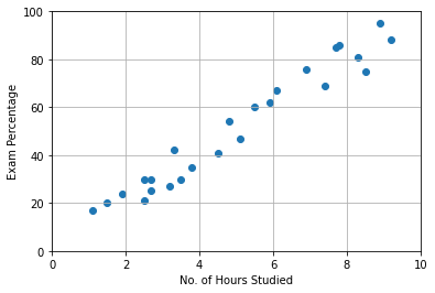
It is a challenging problem to solve analytically. There is no possible way to fit a linear equation to this set of points. The equation that will fit all the points will be all curly, touching each and every point and that is nearly impossible to model. So, we try to find a linear equation that minimizes the squared error.

As we know, the equation of straight line is, y = mx + c

Let’s consider, that line passes through (0,0) for simplicity. So,

y = mx

or

y = x.m

In matrix notation, this problem is formulated using the normal equation,

X^T.X.m = X^T.y

This can be rearranged in order to specify the solution for m as,

m = (X^T.X)^-1 . X^T. y

>>> X = X.reshape(-1,1)
>>> m = np.linalg.inv(X.T.dot(X)).dot(X.T).dot(Y)
>>> m

array([10.17425707])

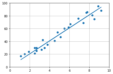
So, the equation that we got after solving for m using normal equation,

y = 10.17425707x

This equation nearly models the actual data as we can see from the graph below.

>>> yadj = X.dot(m)

>>> plt.plot(X,yadj)
>>> plt.scatter(X,Y)
>>> plt.grid()
>>> plt.ylim(0,100)
>>> plt.xlim(0,10)
>>> plt.show()

Let’s take another example,

>>> X = np.array([1,2,3,4])
>>> Y = np.array([5,2,3,1])

>>> X = X.reshape(-1,1)

What happens in this case, according to our solution?

>>> m = np.linalg.inv(X.T.dot(X)).dot(X.T).dot(Y)
>>> m

array([0.73333333])

>>> yadj = X.dot(m)

>>> plt.plot(X,yadj)
>>> plt.scatter(X,Y)
>>> plt.grid()
>>> plt.ylim(0,6)
>>> plt.xlim(0,5)
>>> plt.show()

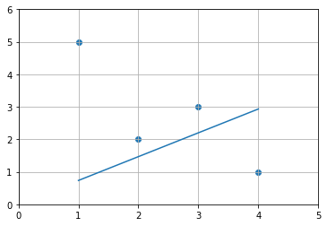
Since, we omitted c from our equation previously, we have a straight line passing through 0. But it neverthless tries to minimize the squared error.

Now, how do we handle the case with c?

5 = m*1 + c*1
2 = m*2 + c*1
3 = m*3 + c*1
1 = m*4 + c*1
 
[[5]     [[1  1]
 [2]   =  [2  1] . [[m]
 [3]      [3  1]    [c]]
 [1]]     [4  1]] 
 
 Y = X . b
 where X consists [1],[1],[1],[1] elements too and b consists of [m],[c] elements.

So,

>>> X_ = np.hstack((X,np.array([[1],[1],[1],[1]])))
>>> X_

array([[1, 1],
       [2, 1],
       [3, 1],
       [4, 1]])

>>> b = np.linalg.inv(X_.T.dot(X_)).dot(X_.T).dot(Y)
>>> print(b)
>>> print(f"m = {b[0]}, c = {b[1]}")

[-1.1  5.5]
m = -1.1000000000000003, c = 5.499999999999999

>>> yadj = X.dot(b[0]) + b[1] # y = mx + c
>>> print(yadj)

[[4.4]
 [3.3]
 [2.2]
 [1.1]]

>>> plt.plot(X,yadj)
>>> plt.scatter(X,Y)
>>> plt.grid()
>>> plt.ylim(0,6)
>>> plt.xlim(0,5)
>>> plt.show()

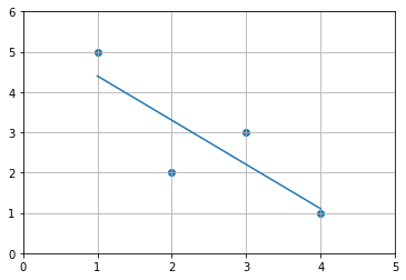
Now, we can see that, the linear equation fits correctly models the data points.